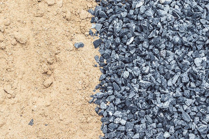
Size and shape of aggregate go a long way in defining what type of concrete will come from mix design
When looking to make improvements on concrete mix design, it is natural to first gravitate to the water-to-cementitious materials ratio, cementitious materials type and amount, admixtures and air content. These are all good considerations, but the mix component that occupies more than 70% of the concrete volume often is overlooked.
Aggregates
These natural particles are the backbone of every good, quality mix. They must be clean, durable and free from deleterious material and supplied in gradations that fall within the parameters of the applicable standard, which typically is ASTM C33 – Standard Specification for Concrete Aggregates or AASHTO equivalents M80 and M6.

Aggregate gradation significantly influences concrete quality. This one characteristic can control a product’s durability and sustainability while having a significant impact on the cost per yard.
However, instead of analyzing the traditional binary blends of fine and coarse aggregates discreetly, producers should go a step further and analyze the gradation of all aggregates together or – in other words – combined aggregate gradation.
This additional analysis results in better fresh concrete workability and overall product quality while potentially saving money.
“Producers need to look beyond price per ton of aggregates,” said Paul Ramsburg, district manager at Sika USA. “Think about it in terms of price per cubic yard or price per finished structure. Spending a little more on sand and stone blends to optimize gradations may result in overall decrease in costs of a cubic yard of concrete that could exceed that initial aggregate investment.”
Terry Harris, director of technical services at GCP Applied Technologies, added: “Some producers are hesitant to look at combined aggregate gradation. Maybe they only have two aggregate bins, so they are limited to one stone and one sand. But there’s still an opportunity to optimize gradation by choosing the best coarse aggregate blend and by choosing the optimal coarse/fine proportions.”
Less is best with paste
Concrete is defined by its individual materials such as fine and coarse aggregates, water and cementitious materials. The two most important for this discussion are aggregates and paste.
Aggregates simply are the total amount of sand and stone in the mix. Paste is cementitious materials, water, air and admixtures. When blended, this liquid surrounds the aggregate particles and guides them through formwork between rebar and blockouts. As it continues to set, it holds sand and stone in suspension to eventually form hardened concrete.
When producing high-quality concrete, strive to use the least amount of paste in order to achieve the plastic properties needed to properly place concrete. For one, paste contains ingredients that are higher priced. And in terms of durability, the majority of potential issues such as shrinkage and deterioration involve paste.
Good concrete needs enough paste to cover the aggregate particles’ surfaces and additional spacing to provide the workability needed to place concrete and consolidate it. That extra room means more paste to provide the workability needed by the fresh concrete matrix. The amount of extra paste depends on a few factors, including the type of aggregates and the paste’s cohesiveness.
“The type of aggregates will have a big impact,” said Jay Shilstone, technical product manager with Command Alkon. “Rough, angular aggregates need more space between particles than rounded aggregates.”
Other factors on combined gradation include formwork complexity and reinforcing along with the desired finish. A product that must be troweled smooth or broom-finished benefits from modifications to the combined aggregate gradation of a concrete that is simply leveled and floated.
The type of concrete will also impact ideal combined gradations. For example, self-consolidating concrete (SCC) performance relies more on optimized combined gradation than conventional or dry cast.
What’s the right amount of paste? There’s no magic number. But performing a combined aggregate gradation analysis is the next best thing.
Avoiding voids
Figure 2 shows a progression that begins with a clear jar filled with large, smooth aggregates. While these aggregates differ in shape, they are around the same size. Note the large air voids between these aggregates.

These voids would have to be filled with paste. Filling the jar with water can give an indication of how empty the voids are.
The second photo shows the addition of a slightly smaller aggregate. While some voids remain, the smaller aggregates find their way among the larger particles to reduce the gaps. Less water – representing less paste – is now needed to fill in.
The third and fourth photos show the addition of even smaller aggregates. Comparing photos 4 and 1 clearly indicates the different amounts of paste needed to fill the voids.
The science behind this phenomenon is called packing. To enhance packing, first examine how fine and coarse aggregates combine to reveal gaps in gradation not visible on traditional, discreet curves. These gaps often exist between the upper end of the fine aggregate and lower end of the coarse aggregate gradations.
To fill that gap, aggregates sometimes are referred to as an intermediate- or medium-sized aggregates that improve aggregate packing. A 2011 study at the University of Toronto titled “Optimization of Aggregate Gradation Combinations to Improve Concrete Sustainability” found that an inclusion of an intermediate-sized aggregate material reduced cement paste up to 16% for a 7250 psi compressive strength mix.
For a project requiring thousands of cubic yards of concrete, 16% is significant.
Methodologies
Throughout this article, the following blend of aggregates will be used and adjusted as an example. Coarse aggregates are a 67 blend along with some manufactured sand. A mix design for 1 cubic yard of concrete has 1,725 pounds of coarse aggregates and 1,367 pounds of sand. The coarse aggregates have a specific gravity of 2.5, and the sand has a specific gravity of 2.6.
To begin analyzing combined aggregate gradation, the percentage of each aggregate by volume must be calculated. Here is an example.
To determine the volume of each aggregate, use this formula:

With these percentages, create a combined aggregate gradation table.

The percentage of each aggregate is shown in light blue.
- Column 1 is the sieve sizes for all aggregates.
- Columns 2 and 3 contain the percentage passing those sieves for the coarse and fine aggregates.
- Column 4 is the aggregates as combined. The formula to calculate the percentage passing each sieve is as follows:
(%CA/100 x %passing CA) + (%FA/100 x %passing FA )
For No. 8 sieve: (0.567 x 2.2) + (0.433 x 98.4) = 43.9%. This represents the total percentage passing from all aggregates.
- Column 5 represents the percentage of total aggregates retained individually on each sieve. It is obtained by calculating the difference in cumulative percentage passing between the current sieve and the next larger sieve.
- For No. 8 Sieve: Individual % retained = 46.0% minus 43.9% = 2.1%
The preceding table represents the most significant step toward optimizing combined aggregate gradation. Recording this data and comparing it to other aggregate deliveries helps measure consistency. It also enables producers to see potential issues in fresh concrete behavior prior to making the first batch.
The data from the previous example can be graphed in a spreadsheet with sieve sizes on the x axis and percentage passing on the y axis. See Figure 3 below.

Some graphical methods of combined aggregate gradation analysis were developed using percentage passing data.
Developed in 1907 and used primarily by the asphalt and concrete industries, the Power 45 curve provides a logarithmic range of sieve sizes on the x axis and the percent passing on the y axis. The gradation results from our previous example have been plotted on this example below. (Figure 4)

The closer the actual gradation curve is to that straight line, the more optimized the gradation.
The Coarseness Chart method was developed in the 1980s by J Shilstone and is based on aggregate proportioning using the combined gradation to proportion a group of sieve sizes that can be categorized as coarse, intermediate and fine aggregates. A coarseness and workability factor is calculated based on the two formulas in this method and plotted on the graph.

Coarseness Factor (CF) =(Q/R)*100
Workability Factor (WF) = W + (2.5(C-564)/94)
- Q = cumulative % retained on the 3/8 Sieve
- R = cumulative % retained on the No. 8 Sieve
- W = % passing the No. 8 Sieve
- C = cementitious material content in lb/yd³
Different zones on the chart delineate aggregate gradations and mix workability (Figure 5). To effectively use the Shilstone Coarseness Chart, select a point in the chart based on the desired properties and back calculate to find the aggregate proportions. This method was not specifically designed for precast concrete mixes, especially SCC.
A graph also can be plotted with individual percentage retained on the y axis versus sieve size on the x axis. Using the previous example, the graph would look like this: (Figure 6)

A few methods of analysis were developed using the graphical system. The Individual Percent Retained Chart – or 8-18 Method – evaluates a distribution of combined aggregate gradation sieve sizes within a given recommended envelope (dotted line) that represent a minimum 8% and maximum 18% retained on each sieve. (Figure 7)

The blue line represents data from the example. Most of the gradation is within the 8-18 envelope, except at the No. 8 sieve. The gap in this size aggregate could be an issue.
Dan Cook and Tyler Ley developed the Tarantula Curve method in 2013 specifically for use with concrete pavements. It is similar to the 8-18 Method, but the envelope is adjusted based on performance testing, comparing the workability of more than 500 different mixtures. (Figure 8)

The resulting upper and lower limits form a shape similar to a spider, thus the name. Developers found that the desirable overall combinations that fall within the Tarantula Curve provide improved workability and resistance to segregation. Once again, the blue line represents the data from the previous example.
Coarse aggregates retained on sieves 1 inch to No. 4 that are near or exceeding the upper range of this curve can increase the risk of segregation and decrease workability. Coarser sands retained on sieves Nos. 8 to 30 play a role in mix cohesion. Too little of this aggregate range could lead to segregation. The finer sands retained on sieves 30 and above impact mix consolidation and finish.
The entire graph from the example data falls within these limits, but that’s no guarantee of optimum performance.
The Tarantula Curve originally was designed for concrete paving and is more suited for conventional concrete mixes. For SCC mixes, the limits will differ. An example of a modified combined gradation curve for precast SCC mixes. (Figure 9)

When comparing this graph to the Tarantula curve, it is evident there is more emphasis on mid-range aggregate sizes. That is due to the fact that having a higher percentage of this mid-range aggregate will produce the optimum performance that SCC requires.
The blue line represents the results from the example data. If this were an SCC mix, the first concern would be lack of intermediate sized aggregates in the No. 4 to No. 8 range.
This could be improved by mixing in another gradation of coarse aggregates and adjusting the percentages. Adding 15% of a No. 89 blend, reducing the No. 67 blend to 50% and reducing the sand percentage to 35%. The new table is:

The resulting modified graphic is show below.

The previous aggregate combined gradation can still be seen in blue, and the adjusted one is in red. Peaks at the high and low end of the combined aggregates were reduced and the larger gap near No. 4 to No. 8 sieves was improved.
At this point, a producer could run a test batch to see how the concrete behaves while mixing, placing and finishing. Fresh and hardened concrete tests could be run and, based on the results, further modifications could be required.
Otherwise, this combined aggregate gradation would be considered optimized for the given materials and conditions.
What to do now?
Starting down the road of optimizing combined aggregate gradation can be daunting, but the payoff makes the effort worthwhile. Check with the admixture supplier for specific methods or programs. Regional admixture representatives are better equipped to help since they are aware of relevant conditions. Nothing beats local knowledge.
Otherwise:
- Create spreadsheets and plot simple gradation charts. Create one for fine aggregate fineness modulus to assess consistency between aggregate deliveries.
- Look for vendors that supply mix design and combined aggregate gradation optimization software.
While combined aggregate gradation methods originated for the paving industry, the precast industry is well-suited for this quality control process because of early-age loading, durability requirements and the wide use of SCC.
Claude Goguen, P.E., is the director of outreach and technical education at NPCA.